Figure
2. Progression of Idea

1. Signal Detection Theory
·
Take a fixed sample
of N observations
{ X1 X2 … XN }
·
Compute the
evidence from the fixed sample
LA
= log { Pr[ {X1 X2 … XN
} | HA)}
LB
= log { Pr[ {X1 X2 … XN
} | HB)}
·
Compare the total
evidence to a criterion
Choose A
if LA – LB > criterion
Choose A
if LB – LA > criterion
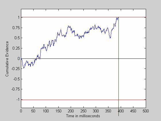
2. Random Walk
·
Sequentially
Sample Observations
o
{ X1 X2
… Xn ...}
·
Cumulate the
evidence online
LA(n+1) = LA(n) + log{Pr[Xn+1 | HA]}
LB(n+1) = LB(n) + log{Pr[Xn+1 | HB]}
·
Decide when
to stop and then what to choose
Stop and choose A if (LA(n+1)
- LB(n+1) > Threshold
Stop and choose B if (LB(n+1)
- LA(n+1) > Threshold
3. What is Gained?
·
Signal Detection
Model
o
Explains Hit and
FA Rates
o
Uses 2 parameters
§
d’ = discriminability
§
b = criterion bias
·
Random Walk Model
o
Explains Hits and
FA rates, plus RT Distributions
o
Uses 3 Parameters
§
d’ = discriminability
§
z = biased starting value (LA(0) - LA(0)
)
§
q = Threshold Bound
4. Speed – Accuracy Trade-Offs
·
The threshold
used in Random Walk Models also provides a direct way of explaining and
measuring speed – accuracy trade off effects
·
Providing more
time to decide tends to produce more accurate decisions
·
Instructions
emphasizing accuracy
·
Deadline Time
Limits
·
Individual
Differences in impulsiveness
5. Discrete Time Stochastic Linear Systems
·
L(n+1) = (1-a)L(n) + V(n+1)
·
V(n+1) = evidence from new observation
·
a = growth – decay parameter
·
V(n+1) = m + e(n+1)
o
m = E[ V(n) ] = mean drift rate
o
Var[e(n+1)] = s2 =
variance
o
d’ = (m / s)
6. Limit to Continuous Time Diffusion
Models
·
t = n∙h h, 2h, 3h, ….
·
L(t+h) = (1-ah) L(t) + V(t+h)
·
V(t+h) = mh + e(t+h)
o
m h= E[ V(t) ] =
mean drift rate
o
Var[e(t+h)] = h s 2 = variance
·
L(t+h)-L(t)
= -ah∙L(t) + m h + e(t+h)√h
o
dL(t+h) = L(t+h)-L(t)
·
dL(t+h) = -ah∙L(t) + m h + e(t+h)√h
·
When we let h
à 0 we get the
§
Ornstein – Uhlenbeck diffusion
model
§
dL(t)
= [m -a∙L(t)
] dt + e(t)√dt