Latent
Structural Equation Models
Purpose: Combine a econometric structural (regression)
model with a psychometric measurement (factor) model.
The structural model is a causal model
that relates the exogenous (independent) variables to the endogenous
(dependent) variables.
The measurement model is a factor
model that relates the observed indicators to the latent factors. All relations
are assumed to be linear.
References:
Bollen, K. A. (1989) Structural
equations with latent variables. NY: Wiley
Long, J.S. (1983) Covariance
structure models: An introduction to LISREL. Beverly Hills: Sage Pubications.
MacCallum,R.
C.; Wegener, D. T.; Uchino, B. N.; Fabrigar, L.R. The problem of equivalent
models in applications of covariance structure analysis.
Psychological-Bulletin.1993 Jul; Vol 114(1): 185-199.
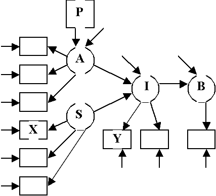
Fishbein Model

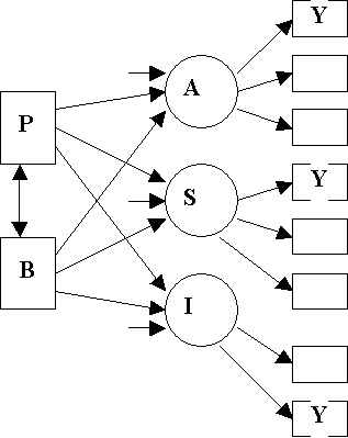
Boxes: Manifest variables
Circles: Latent Variables
Marked Arrows: Hypothesized Causal Relations
Unmarked Arrows: Other Unknown Disturbances or Errors
Double Arrows: Corrlated Variables
Equations
For Fishbein Model
Structural
Equations:
A =
g1P + V1
I =
b1A + g2S + V2
B =
b2×I + V3
Measurement
Equations:
X1
= S + e4
X2
= l3 S + e5
X3
= l4 S + e6
Y1
= A + e1
Y2
= l1 A + e2
Y3
= l2 A + e3
Y4
= I + e7
Y5
= l5 I + e8
Parameters: 23
g1 g2 b1 b2
l1 l2 l3 l4 l5
V(V1) V(V2) V(V3)
V(e1) V(e2) V(e3) V(e4) V(e5) V(e6) V(e7) V(e8)
V(P)
V(S) Cov(P,S)
Bem Model

Boxes: Manifest Measures
Circles: Latent Factors
Equations
For Bem Model
Structural
Equations:
A =
g1B + g2P + V1
S =
g3B + g4P + V2
I = g5B + g6P + V3
Measurement
Equations:
Y1
= A + e1
Y2
= l1 A + e2
Y3
= l2 A + e3
Y4
= S + e4
Y5
= l3 S + e5
Y6
= l4 S + e6
Y7
= I + e7
Y8
= l5 I + e8
Parameters: 25
g1 g2 g3 g4 g5 g6
l1 l2 l3 l4 l5
V(V1) V(V2) V(V3)
V(e1) V(e2) V(e3) V(e4) V(e5) V(e6) V(e7) V(e8)
V(P)
V(B) Cov(P,B)
Modified
Fishbein Model

Equations
For Modified Fishbein Model
Structural
Equations:
A =
g1P + V1
I =
b1A + g2S + V2
B =
b2×I + b3×P + V3
Measurement
Equations:
X1
= S + e4
X2
= l3 S + e5
X3
= l4 S + e6
Y1
= A + e1
Y2
= l1 A + e2
Y3
= l2 A + e3
Y4
= I + e7
Y5
= l5 I + e8
Parameters: 24
g1 g2 b1 b2 b3
l1 l2 l3 l4 l5
V(V1) V(V2) V(V3)
V(e1) V(e2) V(e3) V(e4) V(e5) V(e6) V(e7) V(e8)
V(P)
V(S) Cov(P,S)
Data
Used to Test Models
The
models are evaluated on the bass of their fits to the variance - covariance
matrix.
|
|
P |
X1 |
X2 |
X3 |
X4 |
X5 |
X6 |
Y1 |
Y2 |
Y3 |
|
P |
98.0256 |
0.260437 |
3.655717 |
-3.24522 |
2.011896 |
-3.99883 |
-0.73241 |
0.101508 |
4.245765 |
26.37323 |
|
X1 |
0.260437 |
32.02758 |
8.782259 |
4.513822 |
0.295539 |
-0.10599 |
1.947976 |
7.403358 |
4.578843 |
4.621822 |
|
X2 |
3.655717 |
8.782259 |
33.06517 |
3.426569 |
0.06254 |
2.332248 |
3.35754 |
3.663966 |
4.035624 |
5.569399 |
|
X3 |
-3.24522 |
4.513822 |
3.426569 |
27.92651 |
0.990226 |
0.692618 |
0.839207 |
3.067759 |
1.922617 |
0.886226 |
|
X4 |
2.011896 |
0.295539 |
0.06254 |
0.990226 |
32.05944 |
4.616755 |
-3.31035 |
4.577991 |
4.105686 |
4.590362 |
|
X5 |
-3.99883 |
-0.10599 |
2.332248 |
0.692618 |
4.616755 |
32.78238 |
-2.99564 |
2.835772 |
0.931755 |
1.19207 |
|
X6 |
-0.73241 |
1.947976 |
3.35754 |
0.839207 |
-3.31035 |
-2.99564 |
27.46124 |
-0.84694 |
-0.92867 |
-0.88343 |
|
Y1 |
0.101508 |
7.403358 |
3.663966 |
3.067759 |
4.577991 |
2.835772 |
-0.84694 |
35.57686 |
6.393068 |
5.880421 |
|
Y2 |
4.245765 |
4.578843 |
4.035624 |
1.922617 |
4.105686 |
0.931755 |
-0.92867 |
6.393068 |
30.24919 |
5.518454 |
|
Y3 |
26.37323 |
4.621822 |
5.569399 |
0.886226 |
4.590362 |
1.19207 |
-0.88343 |
5.880421 |
5.518454 |
16.15012 |
10
variables yields (10)*(11)/2 = 55
covariances.
Each
model is fit to the data by searching for the parameters that minimize a discrepancy
function that measures the lack of fit between the predicted and observed
data points.
F(model)
= S S wij [ Covij(obs) - Covij(model) ]2
Under
certain distribution assumptions, for large sample sizes,
(N-1)×F ~ Chi-square
df
= (no. data points - no. parameters)
Nested versus
Non-nested Model Comparisons
Chi-square
comparisons are limited to comparison of nested models.
Model A is nested within
Model B if Model A is a special case of Model B -- Model A constructed by
restricting the parameter space of Mode B.
The Fishbein model
is nested within the modified Fishbein model.
(set b3 = 0).
But the Bem model is
not nested within either of the above.
Cross Validation
This method can be
used for non-nested models that differ in number of parameters.
Divide total sample
into two parts, calibration versus test sample.
N = N1 +
N2
S1 is
the sample cov matrix from first sample
S2 is
the sample cov matrix from second sample
1. Estimate q of each model using S1
.
2. Use these same
parameters to evaluate fit to S2 .
3. Compare each
model using F from second test sample.
4. This procedure
can be repeated many times with different partitions of the data to produce a
sampling distribution for the cross validation index.
5. Under certain
distribution assumptions, it is possible to theoretically derive the cross -
validation estimate. This is a simpler and more efficient method.
Fit Indices
q = no. of measurements
for exogenous var's,
p = no. of measements for
endogenous var's
X = N x (p+q) data matrix, N
= no. observations
S = X'X/(N-1) = (p+q) x
(p+q)
sample covariance matrix
S = predicted covariance matrix
v = (p+q)(p+q+1)/2
s = no.
model parm's
F = .5
Tr [ (S-1(S - S ))2 ] (Generalized Least Squares Lack of Fit)
Indices:
GFI = 1 - 2
F /(p+q)) (Goodness of fit, like R-square)
c 2 = (N-1)F (Chi-square lack of fit)
Cross sample
estimate of F
AIC = c 2 + 2 s (Derived from Information Theory)
BIC = c 2 +
ln(N) s (Derived from Bayesian
Statistical Theory)
Choose the
model with the highest GFI
or lowest
cross sample F, Chi-square, AIC, or BIC .
Model
Comparisons
|
Model |
parm's |
Chi-Sq |
Cross-F |
AIC |
BIC |
GFI |
|
Fish |
23 |
79.4*** |
(.20,
.31) |
125 |
-9 |
.968 |
|
Bem |
25 |
51.0* |
(.16,
.24) |
101 |
-25 |
.980 |
|
M-Fish |
24 |
30.3 |
(.12,
.19) |
78 |
-52 |
.988 |
Note:
Cross validation column displays 90% confidence interval.
* p
< .05 ** p < .01 *** p < .001
Based
on this analysis, we would choose the Modified Fishbein Model.
Concluding
Comments About Model Comparisons in General:
1.
Chi-square tests are limited to nested model comparisons.
2. Non-nested
model comparisons are more important.
3.
Cross validation provides an important tool for non-nested model comparisons.
4.
Model evaluation is meaningless without performing critical model comparisons.